

Consider a month-end report that returns one row of totals, a support dashboard with two small tiles, and an assistant that answers "how many orders in region R3?" with a single number. Each of them is correct, each is slower or busier than it should be, and each has a proposed fix waiting in a pull request: a bigger memory grant, a new index, a nightly statistics job, a faster refresh. The plan that SQL Server actually ran is usually not attached to any of them.
The question most engineers arrive with is simple: this query, this report or this server is slow, so what should I read before I change an index, a hint or a job? This guide draws the map. Seven deep dives on DevInside each measured one part of it on SQL Server 2025, each with a solution you can download; here their numbers sit side by side, and every section ends with the article that answers the next question.
- The optimizer decides the plan shape and the memory grant once, from estimates built on statistics. An actual plan shows where those estimates were wrong; tuning starts from that difference, not from the operator names.
- Rows returned says nothing about the work. Read rows read against rows passed on: a typed parameter read 6,250 index rows for an answer that an inferred
nvarcharparameter reached by reading 50,002. - A spill is a fixed grant running out, and its cause can be the size of each row rather than the row count. Shrinking the grouping key cut a report from 471 ms to 89 ms; a bigger grant made 16 concurrent reports wait seconds for memory.
- Observing and maintaining the server are workloads with results of their own. Twenty dashboards cut business lookups from 1,579 to 186 a second; a statistics job reported success 40 times while 9 runs missed their goal; a naive cutover lost 217 to 362 confirmed invoices per run.
Estimates are made once, and everything after runs on them
Every topic in this guide hangs off one sequence. Statistics describe the data. The optimizer turns them into row estimates, and from those it picks a plan and sizes the memory the plan may use. Execution then reads rows, fills the grant, sometimes writes to tempdb, and leaves runtime numbers behind for Query Store. Around that loop sit the people and jobs that watch the server and keep it healthy. Where does each kind of problem enter, and where can you see it?
Statistics feed the estimate, and the estimate fixes the plan and the grant before the first row
- The whole cast. The top row is one query, from statistics to rows read; the rest are the things that learn from it, watch it or keep it healthy.
- Statistics are the optimizer's only picture of the data. With 1,000 new orders above the last histogram step, it estimated 50 rows for a category that held 1,000.
- From the estimates it picks the plan shape and the memory grant before the first row is read: 28,120 KB for the month-end report, and the grant cannot grow later.
- Execution reads what the plan's seek keys allow and throws away what a residual predicate rejects. When the hash table outgrew its grant, 2,202 pages went to tempdb and back.
- Query Store keeps the actual numbers, and memory grant feedback hands them to the next compile: the same report got 63,880 KB on its second execution and stopped spilling.
- Every dashboard tile and diagnostic poll is a query on the same server. One status tile read 546 pages per refresh; a business lookup read 2.
- Maintenance and recovery change the inputs of all of this. A job that reports success has not proved its statistic changed, and a restored database has not proved the application works.
Mechanism as described in Microsoft's cardinality estimation, statistics and memory grant documentation. Values from the sql-diagnostics, hash-spills and sql-monitoring-cost solutions on SQL Server 2025 (17.0.5065.9, RTM-CU11).
The figure has one asymmetry worth remembering. Everything on the top row is decided before execution starts, and execution has no way to renegotiate it: a plan chosen for 50 rows runs its key lookups 1,000 times, and a grant sized for one estimate stays that size. That is why the first diagnostic move is always the same. Capture an actual plan, find the operator where estimated and actual numbers part, and ask which input produced the estimate.
The optimizer chooses from estimates, and statistics are its picture of the data
SQL Server's optimizer is cost-based: it picks the plan with the lowest estimated cost, and the main input to that cost is the number of rows expected at each operator. Those cardinality estimates come primarily from histograms built when statistics are created or updated (cardinality estimation). A histogram has at most 200 steps over the leading column of a statistic, plus density information for column prefixes, computed at one moment and then left alone until something refreshes it.
Automatic updates do not fire on every change. For a table of more than 500 rows the threshold is the smaller of 500 + 0.20 x n and the square root of 1,000 x n modifications to the leading column (Statistics). For 10,000 rows that is 2,500. In the maintenance deep dive, 1,000 orders arrived in a new category 99, above the histogram's last step and below the threshold. The optimizer estimated 50 rows, chose an index seek with key lookups, ran them 1,000 times and read 2,076 pages of a table with 306 data pages. After a qualified UPDATE STATISTICS ... WITH FULLSCAN the estimate was exact, a clustered index scan won, and the same query read 308 pages.
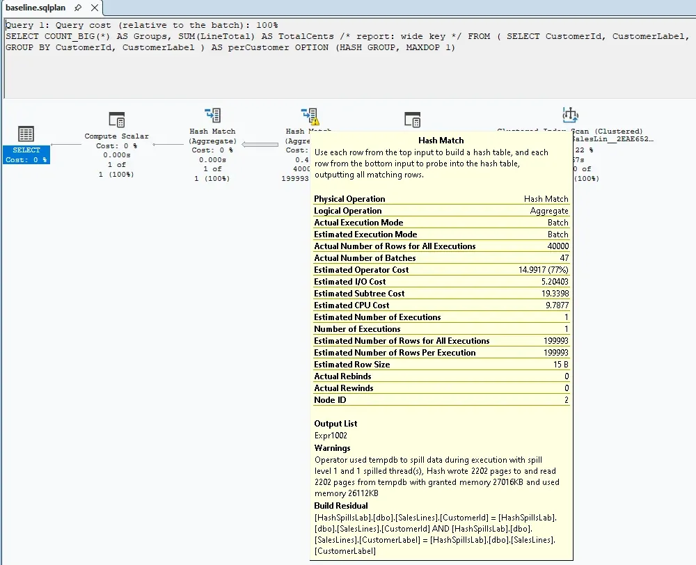
An estimate has two parts, though, and statistics only fix one of them. In the hash spill lab the optimizer overestimated a report's groups fivefold (199,993 against 40,000) and still spilled, because it assumed about 0.14 KB per group where each group really needed about 1.4 KB. Multi-column statistics made the group estimate exactly 40,000; the grant fell from 28,120 to 10,008 KB and the spill grew from 2,202 to 4,014 pages each way. The classic case does exist: with statistics frozen at 1,000 customers, the same kind of aggregate spilled at level 2 and took 1,686 ms at the median, and an update with a full scan brought it to 366 ms. So "update statistics" is the right fix when the row count was underestimated, and the wrong reflex when the plan already overestimated it.
Statistics also change under you. The maintenance lab recorded the engine's own automatic update replacing a full-scan statistic on a 300,000-row table with a 17.7% sample, with no job involved, and ALTER INDEX ... REORGANIZE leaving a statistic with 5,000 pending changes where REBUILD refreshed it. A policy that says "full scan" needs a check that reads rows_sampled, not a schedule.
Read this next: SQL maintenance and diagnostics as products shows the histogram before and after the update, the sampling table step by step, and a verifier that judges the statistic you meant rather than the one the job touched.
An actual plan says how much was read, not only what came back
Most slow queries in an application return small results. The work is elsewhere, and the actual plan records it on the access operator in three numbers. ActualRowsRead is how many index or table rows the operator examined. ActualRows is how many it passed on after its residual predicate. The result set is what the client finally sees. The operator name, "Index Seek" or "Index Scan", tells you none of them.
What decides rows read is the split between seek keys and residual predicates. A seek key narrows the range the engine walks in the index. A residual predicate is tested on every row inside that range and throws away the ones that fail. In the agent deep dive, a tool asked for the orders of one tenant in region R3. Bound as varchar(8), the column's own type, both TenantId and RegionCode were seek keys: 6,250 rows read, 30 logical reads. Sent the AddWithValue way, the same value arrived as nvarchar(2). Data type precedence converted the column side, CONVERT_IMPLICIT moved the region test into the residual, and the seek walked the whole tenant: 50,002 rows read, 217 logical reads, for the same 5,625 rows passed on and the same one-row answer. The tool path's median went from 8.35 to 22.7 ms.
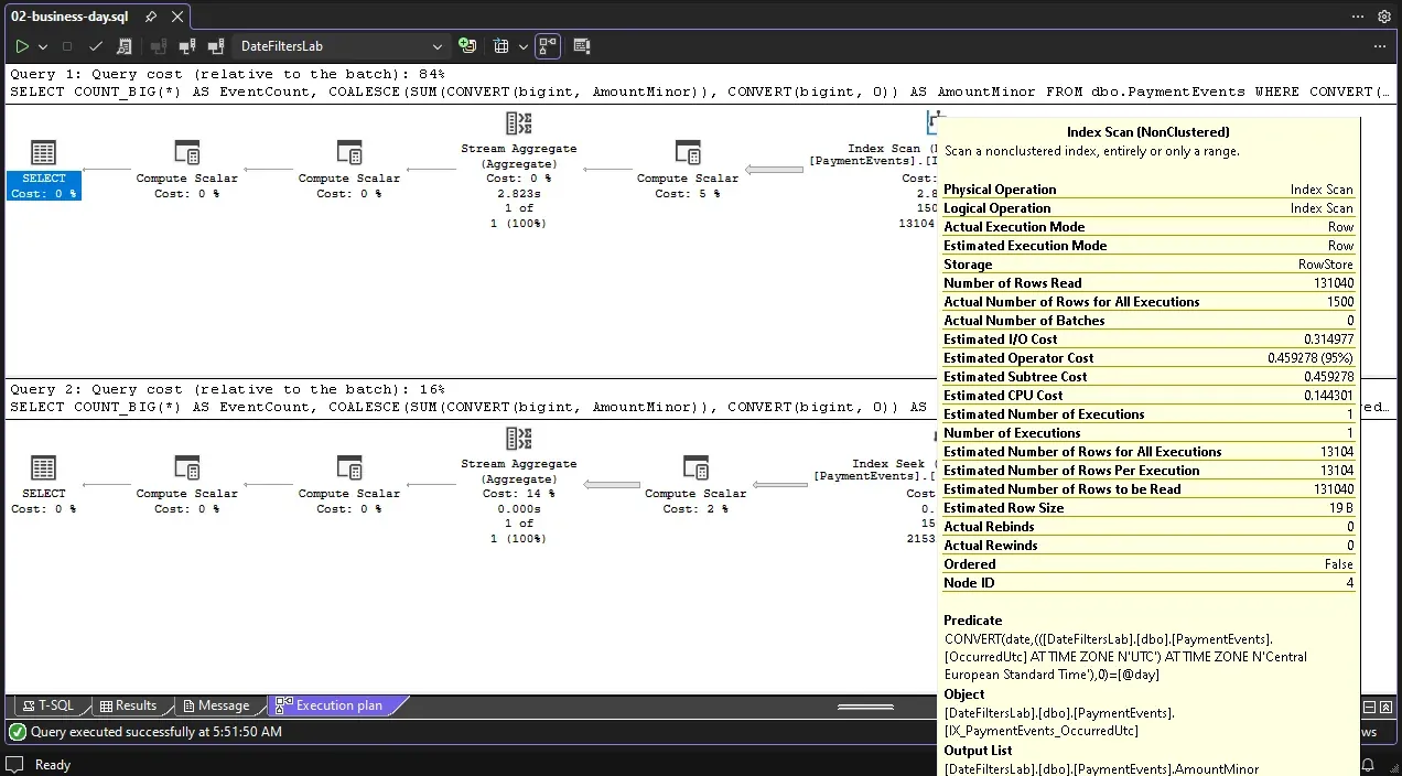
Date filters show the same split on the most common predicate in reporting. In the date-filter deep dive, a table of 131,040 payments was asked for 26 October 2025 in Warsaw, a 25-hour day. The half-open interval OccurredUtc >= @start AND OccurredUtc < @end, with both boundaries sent as typed datetime2(7) values, seeked and read exactly the 1,500 rows it returned: 9 logical reads, 2.5 ms at the client median. CONVERT(date, OccurredUtc) still produced an Index Seek, but its dynamic range read 2,880 rows to pass on 1,440, was estimated at one row and answered the UTC day instead of the Warsaw day. Converting the column with AT TIME ZONE gave the right answer by scanning all 131,040 rows, 426 logical reads and 2,363 ms at the median, against 2.6 ms for the same conversion applied to the two boundaries.
The same rule decides whether an index is used at all. In the JSON deep dive, a computed column RegionKey AS TRY_CONVERT(int, JSON_VALUE(Document, '$.region')) with an index served the dashboard query in 3 logical reads and 10.1 ms at the median. The identical expression typed with bigint returned the same 100 orders and scanned all 3,239 pages, 267 ms at the median, because the optimizer matches the expression in the index definition literally. On the build tested, the new JSON index served JSON_CONTAINS (319 reads) but not JSON_VALUE equality, which scanned, although the documentation lists it. The plan is the acceptance test; the feature description is not.
Two habits follow. When a seek reads far more than it passes on, open its seek keys before adding an index, and look for CONVERT_IMPLICIT on a column. And when you cannot capture plans in production, Query Store still helps: it has no rows-read counter, but in the agent lab the two bindings appeared as two queries with average logical reads of 30 and 217, and only the second stored plan contained CONVERT_IMPLICIT.
Read this next: SQL date filters reads rows read from the actual plan of every predicate and tests each against events placed on the local midnights; An AI agent on SQL Server walks the seek operator attribute by attribute and times the tool path stage by stage; Indexing JSON measures which predicates use which index and what each index costs on writes.
Memory is granted before the first row, and a spill is the grant running out
Sorts, hash joins and hash aggregates need workspace memory, and they get it as a query memory grant: a reservation sized at compile time from estimated rows times estimated row size, taken from a resource semaphore that every concurrent query shares (memory grant troubleshooting). The optimizer computes a required amount, the minimum to start, and a desired amount, what it believes avoids spilling. By default one query may take at most 25% of what can be granted. Once granted, the amount is fixed. When a hash table outgrows its share, the operator writes partitions to tempdb and reads them back; each further round is another spill level.
The month-end report in the hash spill deep dive shows how to read it. The plan asked for 28,120 KB, got all of it, used 26,336 KB and spilled 2,202 pages at level 1: 471 ms at the median. Five numbers on the spilling operator and the plan root told the story: estimated against actual groups, desired against granted memory, maximum used memory, execution mode, and pages written to tempdb. They also ruled out the popular fixes. A MIN_GRANT_PERCENT = 20 hint removed the spill alone (271 ms) but is a percentage of a moving maximum: under concurrency every copy got the estimate's 28,120 KB and spilled anyway. Sixteen wide-key reports at once took 7.3 s at the median, five waited on RESOURCE_SEMAPHORE for up to 5.6 s, and sixteen copies with the minimum grant did not finish within 30 s.
The fix that held was making the state smaller. Grouping by the narrow customer key and joining the label afterwards needed 3,560 KB for the aggregate, never spilled and took 89 ms at the median; with 16 reports at once it waited at most 53 ms for memory and finished every report within 1.6 s. Before tuning at all, run the query again: memory grant feedback raised the cached plan's grant to 63,880 KB on its second execution, and with Query Store persistence it reached even an OPTION (RECOMPILE) statement from its third.
Read this next: Hash aggregates, parallel plans and memory grants slides through five grant sizes, reads the memory broker while the report runs and measures 8 and 16 reports released together.
Watching the server is a workload, and it has a plan too
Every number in the previous sections came from looking at the server, and looking is not free. A monitoring query is optimized, granted memory and executed like any other, and its cost is per call times refresh rate times the number of people watching. In the monitoring deep dive, a size tile reading sys.dm_db_partition_stats cost 9 logical reads, an exact COUNT_BIG(*) cost 546, every page of the table, and a business lookup cost 2. With four lookup workers and twenty dashboards each querying once a second, lookups fell from 1,579 to 186 a second and their p99 rose from 17.5 to 105 ms. One server-side refresher sharing a snapshot left them at 1,643 a second.
Locks are the less visible cost. Under the default read committed isolation without row versioning, the counting tile waited on a writer's row lock, and an unrelated writer then queued behind the waiting tile: sys.dm_exec_requests named the dashboard as the blocker. A lock timeout shorter than the refresh interval, or reading row versions, keeps a monitor out of the queue. The shape of a diagnostic query matters as much as its frequency. Shredding an Extended Events ring buffer inline cost 10.1 to 11.6 s of CPU per poll of 200 events; reading the same events from an event file by offset cost 19 to 40 ms. And Query Store's default capture mode undercounts light, frequent queries: 100 metadata tiles were recorded as 71 executions.
sys.dm_exec_requests names the dashboard as the blocker; writer D waits with LCK_M_IX behind its LCK_M_S and gives up after 2,009 ms. Timings vary between runs.Diagnostics you build yourself follow the same arithmetic. In the maintenance lab, checking one statistic cost 1.6 to 2.3 ms of server CPU at the median, cheap enough to run after every step. A sweep over 312 statistics cost 771 ms of CPU when it called the per-statistic collector in a loop and 107 ms as one set-based statement.
Read this next: When monitoring becomes the workload builds the shared snapshot with a lock timeout and a visible age, and measures the blocking chain, the indexed view alternative and the common diagnostic polls.
Maintenance and recovery succeed only when you check the result
The operations side changes the inputs everything above depends on, and it fails quietly. A completed command proves that the command ran. In the maintenance deep dive, a job built UPDATE STATISTICS Orders ... without a schema, ran as a user whose default schema was archive, and updated archive.Orders while the report's sales.Orders stayed stale. In a seeded workload of 40 runs, the job reported success 40 times and 9 runs failed their postcondition: a one-part name, a reorganize instead of an update, a NULL mode that fell back to a sample, a zero sample that left no histogram. The check that catches it snapshots the statistic by object_id and stats_id before the step and judges the same identity afterwards. Versioned and tested on eleven seeded states, the first diagnostic was right 5 times out of 11 and the third 11 out of 11.
Recovery has the same gap between a green check and a working system. In the recovery deep dive, a backup taken with checksums verified, restored, came online and passed DBCC CHECKDB, and the billing service still could not issue an invoice: its login was missing, a synonym pointed at a database nobody restored, a template file lived on the old site's share, and the restored sequence would reissue an invoice number a customer already held. A runbook written as code, where each step checks its own result and its inputs against live state, recovered the application in 12.5 to 15.3 s per drill, median 13.7 s, on a 252,000-invoice database. Restore and recovery took 3.2 to 4.2 s of that; CHECKDB, reconciliation against an outside journal and the probe took 8.0 to 10.1 s.
A planned move adds one more trap. Pointing the connection name at the new server while the old one stays writable lost 217 to 362 confirmed invoices per run with a 2 s name TTL, and 157 to 187 with a TTL of zero. Fencing the old writer first with a tail-log backup WITH NORECOVERY lost none in five runs, at the price of a 7.1 to 8.5 s pause.
Read this next: SQL Server recovery you can rehearse opens the log chain by LSN, scripts logins by SID, runs a runbook that refuses wrong steps and measures both cutovers.
The measured numbers, side by side
Before the table, one comparison that runs through four deep dives: a fix that did not change the answer, only the work behind it. Each pair below answered the same question with the same rows (the metadata count is an approximate size); only the logical reads changed.
Same answer, very different work: logical reads before and after each fix
| Query (deep dive) | Before | After |
|---|---|---|
| JSON filter, 100 orders | 3239 | 3 |
| Stale statistics, 1,000 orders | 2076 | 308 |
| Size tile, 1 row | 546 | 9 |
| Agent tool, 1 row | 217 | 30 |
- Logical reads of the first version. Every query returned a correct result; nothing in the result hinted at the work behind it.
- The same results after the fix. None of the four fixes added hardware, a hint or a grant.
- These two fixes only made the query match the index: the computed column's own expression, and a parameter typed like the column. No index was added.
- After the statistics update the optimizer chose a scan instead of 1,000 key lookups. The better plan reads every page once.
- The metadata count is approximate by definition. It answers "is the table growing?", not a reconciliation, and it is multiplied by every refresh and every viewer.
Logical reads from SET STATISTICS IO as published in the deep dives: JSON indexing (TRY_CONVERT bigint against int spelling), maintenance and diagnostics (stale statistics against a qualified FULLSCAN), monitoring cost (COUNT_BIG against sys.dm_db_partition_stats), AI agent (nvarchar(2) against varchar(8) parameter). SQL Server 2025 RTM-CU11, warm cache; reads were identical across runs.
Every number below is quoted from the published deep dive in the first column, which takes it from its solution's results/ folder. All runs used SQL Server 2025 Developer (17.0.5065.9, RTM-CU11) in Docker containers capped at 2 GB and 1.5 CPUs, or 3 GB and 2 CPUs for the date-filter, maintenance and recovery labs, on a shared Windows Server 2022 host. Reads, pages and grants are exact and repeated in every run; times move between runs, so compare within a row.
| Deep dive | What was measured | Result |
|---|---|---|
| Maintenance and diagnostics | Report on category 99 with stale statistics against after a qualified FULLSCAN: estimated rows, logical reads | 50 and 2,076 against 1,000 and 308 |
| Maintenance and diagnostics | Seeded maintenance workload: runs reported successful, runs that failed the postcondition | 40 of 40; 9 |
| Maintenance and diagnostics | Correct verdicts on eleven seeded states, diagnostic version 1 against version 3 | 5 of 11 against 11 of 11 |
| Maintenance and diagnostics | CPU for one statistic check (p50); sweep of 312 statistics, loop against one statement | 1.6 to 2.3 ms; 771 ms against 107 ms |
| Hash spills | Wide grouping key: grant, used, spill, p50 | 28,120 KB, 26,336 KB, 2,202 pages, 471 ms |
| Hash spills | Exact group estimate from multi-column statistics: grant, spill, p50 | 10,008 KB, 4,014 pages, 463 ms |
| Hash spills | Narrow key, label joined afterwards: aggregate memory used, p50 and p95 | 3,560 KB, no spill, 89 ms and 117 ms |
| Hash spills | Memory grant feedback, second execution | 63,880 KB, no spill |
| Hash spills | 16 reports at once, p50: wide key against narrow key | 7,287 ms against 1,351 ms |
| Date filters | 25-hour Warsaw day on 131,040 payments, typed half-open interval: rows read, logical reads, client p50 | 1,500, 9, 2.5 ms |
| Date filters | CONVERT(date) on the column: estimated rows, rows read, rows passed on | 1, 2,880, 1,440 (the UTC day) |
| Date filters | AT TIME ZONE on the column against on the two boundaries: rows read, client p50 | 131,040 and 2,363 ms against 1,500 and 2.6 ms |
| Date filters | Predicates that kept every edge event on the right day | 6 of 13 |
| JSON indexing | Computed-column index, matching spelling against bigint spelling: reads, p50 | 3 and 10.1 ms against 3,239 and 267 ms |
| JSON indexing | JSON index with JSON_CONTAINS: reads, p50 | 319, 14.7 ms |
| JSON indexing | Log for a 100-row note change: no index, computed column, JSON index | 15.7, 38.5, 84.5 KB |
| JSON indexing | Index rebuild p50: computed column against JSON index | 122 ms against 4,373 ms |
| AI agent on SQL Server | Rows read at the seek and logical reads, varchar(8) against nvarchar(2) parameter | 6,250 and 30 against 50,002 and 217 |
| AI agent on SQL Server | Tool path p50, same two bindings | 8.35 ms against 22.7 ms |
| Monitoring cost | Logical reads per call: metadata count, exact count, business lookup | 9, 546, 2 |
| Monitoring cost | Lookups per second and lookup p99: no dashboard, 20 viewers querying, shared snapshot | 1,579 and 17.5 ms; 186 and 105 ms; 1,643 and 13.8 ms |
| Monitoring cost | CPU per poll of 200 Extended Events: ring buffer inline against event file | 10.1 to 11.6 s against 19 to 40 ms |
| Recovery | Drill from first step to a working probe, ten runs; of which CHECKDB, reconcile and probe | 12.5 to 15.3 s (median 13.7 s); 8.0 to 10.1 s |
| Recovery | Confirmed invoices lost per cutover run: naive TTL 2 s, naive TTL 0 s, fenced | 217 to 362, 157 to 187, 0 |
| Recovery | Pause without confirmations in the fenced cutover | 7.1 to 8.5 s |
Read down the result column and the argument of this guide is in the data. The large wins came from making a query match its index, giving the optimizer a true picture of the data or shrinking the state a plan must hold. The expensive surprises came from things that reported success: a green job, a valid backup, a cutover with zero client errors, a dashboard that only returns four rows.
Read this next: one deep dive per question
- "The plan has a spill warning. Do I need more memory?" Read Hash aggregates, parallel plans and memory grants. You get the lab, the saved actual plans and SSMS captures; the key finding is that the size per group, not the group count, was wrong, and that a narrower key beat every grant under concurrency.
- "My query returns one row. Why is it slow?" Read SQL date filters: keep the business day and count the rows read. It tests thirteen predicates for one business day against events placed on the local midnights and reads rows read from every actual plan; the key finding is that a
CONVERT(date)seek read 2,880 rows for 1,440 on the wrong day, while the typed half-open interval read exactly the 1,500 it returned. - "Should I index a JSON property, and which way?" Read Indexing JSON. It opens the JSON index's internal table and measures reads, log bytes and rebuild time for three designs; the key finding is that every document update maintains the index, even when the indexed value does not change.
- "An application or an AI agent sends SQL. How do I know what it costs?" Read An AI agent on SQL Server. It ships a solution with a read-only login, rows-read measurements and Query Store checks; the key finding is that one inferred parameter type read eight times the index rows with every answer still correct.
- "Is our monitoring making things worse?" Read When monitoring becomes the workload. It measures tiles, viewers, blocking and diagnostic polls with terminal captures; the key finding is that a shared snapshot made the database cost independent of how many people watch.
- "The statistics job is green. Are the statistics current?" Read SQL maintenance and diagnostics as products. It seeds eleven states and a 40-run workload and versions the diagnostic that judges them; the key finding is that 9 successful runs missed their postcondition.
- "Our backups verify. Can we recover?" Read SQL Server recovery you can rehearse. It recovers an application on a second instance with a runbook that refuses wrong steps; the key finding is that fencing the old writer, not a shorter TTL, is what stopped lost invoices.
If the time turns out to be in the application rather than the database, what a performance diagnostic should deliver follows one endpoint through profilers and counters to the index that fixed it.
Decision guide: from what the plan shows to the first move
| What you see | First move | What not to do yet |
|---|---|---|
| Estimated rows far below actual on the access operator | Check the statistic's modification_counter, sampling and whether new keys lie above the last histogram step; update it with the sampling your policy requires | Add an index or a join hint for the bad plan |
| Estimated rows far above actual, yet a spill | Divide used memory by actual rows to get the size per row or group; narrow the key or the row | Update statistics and expect the spill to go |
| A seek with rows read far above rows passed on | Read its seek keys and residual predicate; look for CONVERT_IMPLICIT and type parameters like the column | Trust the word "Seek" |
A function or AT TIME ZONE on a filtered column | Compute the two boundaries in the application and filter with a typed half-open interval | Accept the plan because it says Index Seek |
| A scan where you expected an index | Compare the predicate with the index definition character by character; test it in an actual plan | Assume the feature list means the index applies |
| A spill on the first execution | Run the query twice more and check memory grant feedback and Query Store feedback rows | Add MIN_GRANT_PERCENT without a concurrency test |
Grant waits (RESOURCE_SEMAPHORE) rather than spills | Reduce the state each query holds | Raise one query's grant |
| A dashboard or poll among the top queries | One shared refresher with a lock timeout; metadata for sizes; event files read by offset | Lower the refresh rate and stop there |
| A green maintenance job, a stale plan | Snapshot the intended statistic by identity before the step and judge it after | Trust the job log |
| A verified backup | Rehearse recovery to a probe that performs the real operation under the service login | Call the database recovered at ONLINE and a clean CHECKDB |
Checklist
- Capture an actual plan, not an estimated one, and find the first operator where estimated and actual rows part.
- On access operators, compare rows read, rows passed on and rows returned; read the seek keys and the residual predicate.
- Bind every parameter with the column's type and length; check plans or Query Store for
CONVERT_IMPLICITon columns. - For spills, read desired, granted and used memory, the execution mode and tempdb pages before choosing a fix; rerun to see feedback.
- Test grant hints and large grants under the concurrency the query really sees.
- Treat every dashboard tile and diagnostic poll as a query with a cost per call, a refresh rate and a viewer count.
- Judge maintenance on the statistic's identity, timestamp and sampling after the step, not on the job's exit code.
- Rehearse recovery to the application's real operation, and fence the old writer before any endpoint moves.
Further reading
- Cardinality estimation: the cost-based optimizer, histograms as the source of estimates, and the model assumptions.
- Statistics: histograms, automatic update thresholds and when the optimizer checks for out-of-date statistics.
- Troubleshoot memory grant issues: required and desired memory, resource semaphores and RESOURCE_SEMAPHORE waits.
- Memory grant feedback: batch, row, percentile and persistence modes.
- Showplan logical and physical operators reference: seeks, scans and hash operators.
- Data type precedence: why a varchar column is converted when compared with an nvarchar value.
- Transaction locking and row versioning guide: lock compatibility and READ_COMMITTED_SNAPSHOT.
- Tail-log backups: NORECOVERY and the restoring state.