One Row Returned, a Large Intermediate Workload
Two SQL queries return the same one-row aggregate. Actual plans, logical reads and a bounded experiment reveal very different source work.
Explore the mechanism ↓
Reading tools Listen or translate
Read aloud
Uses an installed voice on your device.
Translate article
Machine translation. Code and evidence notes stay in English.
Original English text.
START WITH THE MECHANISM
Interactive companion and laboratory update: 12 November 2026. The editorial date places the topic on the timeline; this current explanation and its measured evidence retain their actual preparation and execution dates.
THE FULL INVESTIGATION
One Row Returned, a Large Intermediate Workload
Dates and technology context
This is a retrospective editorial timeline. Topic context: 9 April 2026. First publicly available: 12 November 2026. Current text, visuals and laboratory revisions were prepared on 12 November 2026.
The 100,000-event fixture, actual rows-read/logical-read counts, plans and timings were executed 2026-11-12. Do not attribute the chosen patch or execution results to the historical core.
A query returns one row. The API serializes a tiny response. The application team concludes that the database work must also have been small.
That conclusion confuses output size with execution work. A single aggregate can sit at the end of a large scan, a repeated lookup or an unexpectedly expanded intermediate result. The final row tells us what the client receives. It does not tell us how much the engine had to inspect before producing it.
This article follows a deliberately simple example: two SQL Server queries calculate the same daily count and amount sum from 100,000 synthetic events. Both return one row containing identical values. Their actual plans read very different numbers of source rows, and their logical-read counts differ substantially.
The experiment was executed on 12 November 2026 against SQL Server 2022 Developer Edition, build 16.0.4315.2. The client uses .NET 9.0.4 and Microsoft.Data.SqlClient 5.1.6. All observations belong to that local laboratory, with its settings and limitations. No customer workload or production incident is implied.
The central lesson is not to ban a particular SQL function or operator. It is to follow the work from the requested result backward through the actual execution, then change the query only while preserving the question it answers.
Define the day before optimizing the predicate
01 / See the idea
Make the interval part of correctness
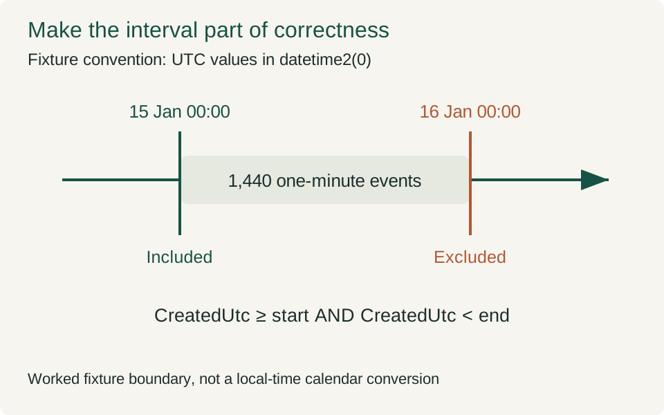
The generated sequence contains events at both boundaries. An inclusive end would select an extra event and fail the independent expected aggregate.
Interpretation and evidence
- Define the time convention.
- Include the lower boundary.
- Exclude the following midnight.
The fixture records event timestamps in a column named CreatedUtc. The column is datetime2(0), not a time-zone-aware type. The experiment treats all values as UTC by convention and generates them from one explicit starting instant.
The business-shaped question is: how many events occurred on 15 January 2025, and what is the sum of their integer amounts? The intended interval begins at that day's midnight and ends immediately before the next midnight.
That definition is not optional decoration. A query that becomes faster by selecting a different time interval is not an optimization of the same operation. Inclusive end bounds, local time conversion and fractional seconds can all change the answer while leaving the SQL superficially similar.
The generated event for identifier id occurs id minutes after 1 January 2025 at midnight. Its amount is id % 1000 + 1. A separate C# oracle applies the specified interval directly to that mathematical sequence. It expects 1,440 matching events and an amount sum of 667,920.
Those expectations are not derived by asking the original SQL query to certify the new SQL query. They are calculated independently from the fixture definition. The two SQL implementations must match the oracle before their plans or timings become relevant.
The interval deliberately includes generated events exactly at both boundaries. The event at the opening midnight belongs in the answer; the event at the following midnight does not. That makes an accidental inclusive upper bound visible in the result rather than leaving it as an untested theoretical concern.
A small schema is enough to expose the mechanism
The event table has three columns and a clustered identifier key:
CREATE TABLE dbo.Events
(
 Id int NOT NULL CONSTRAINT PK_Events PRIMARY KEY,
 CreatedUtc datetime2(0) NOT NULL,
 AmountMinor int NOT NULL
);

CREATE INDEX IX_Events_CreatedUtc
ON dbo.Events(CreatedUtc) INCLUDE(AmountMinor);
The date index includes the amount needed by the aggregate. The query can therefore obtain the relevant timestamp range and amount without fetching a separate wide document. This is an intentional access design, and it belongs in the experiment's input description.
The table contains 100,000 rows, not a fictional million. That size is sufficient to produce an observable access-path difference without turning the exercise into artificial stress on the shared machine. The synthetic distribution is regular, so it does not represent every production event stream.
The laboratory shares a generated dataset and container wrapper with a separate article about indexing JSON. Those other tables are not joined by these queries. Sharing the fixture reduces repeated infrastructure work; it does not combine the two articles' claims. Here the subject is the relationship between a date predicate, the selected access path and the work behind a one-row result.
Statistics are updated after loading, and both queries specify MAXDOP 1. The comparison is therefore about these serial access paths. It does not establish the effects of parallel execution, stale statistics or competing sessions.
The index definition is part of the contract too. A query rewrite cannot seek through an index that does not exist. If a production system has only a different key order or lacks the included amount, its resulting plan may perform additional work that this fixture does not exercise.
Two ways to ask for the same date
The first query converts every timestamp to an eight-character date representation before comparing it with a parameter:
SELECT COUNT_BIG(*) AS MatchCount,
       SUM(CAST(AmountMinor AS bigint)) AS AmountSum
FROM dbo.Events
WHERE CONVERT(char(8),CreatedUtc,112)=@dateText
OPTION(MAXDOP 1);
The parameter is the explicitly typed character value 20250115. Style 112 identifies the particular date representation used by this example. That exact style is important: a language-dependent formatted date would add another source of ambiguity. Microsoft: CAST and CONVERT
The second query expresses a range over the stored timestamp:
SELECT COUNT_BIG(*) AS MatchCount,
       SUM(CAST(AmountMinor AS bigint)) AS AmountSum
FROM dbo.Events
WHERE CreatedUtc>=@date
  AND CreatedUtc<DATEADD(day,1,@date)
OPTION(MAXDOP 1);
The parameter is midnight on 15 January 2025, supplied as datetime2. The upper bound is exclusive. This avoids inventing a last representable instant of the day and makes the intended interval visible in the predicate.
The range shape gives the optimizer an opportunity to use the timestamp ordering directly. The actual plan, rather than the query's appearance, establishes whether that happened in the tested configuration.
Do not turn this example into a universal rule that every function applied to a column prevents a seek. SQL Server can transform some expressions and derive useful ranges in ways that are not obvious from source syntax. The experiment demonstrates this particular conversion and this particular range, with actual evidence for both.
The reverse slogan would be just as misleading. A predicate that looks index-friendly does not guarantee that an index seek is the best or selected plan. Selectivity, coverage, estimates and other work still matter. The word seek is a description of an operation, not a certificate that the query is efficient.
The client supplies types, not just strings
The C# harness uses parameter objects rather than constructing a SQL statement by concatenating values. These are the actual parameter assignments for the two date inputs:
q.Parameters.Add("@dateText",SqlDbType.Char,8).Value="20250115";
q.Parameters.Add("@date",SqlDbType.DateTime2).Value=new DateTime(2025,1,15);
The source retains the parameter types alongside the SQL. A parameter's type can influence conversion and plan behavior; it should not be an accidental detail hidden inside a helper that guesses from a string.
The reader drains all result sets. In a diagnostic execution, that includes the actual-plan XML as well as the aggregate row. In a timed execution, plan collection is disabled, and the timer covers command execution through result draining.
That boundary is narrower than a complete HTTP request and wider than an isolated engine operator. It includes the local client/server exchange and the small result reader. It excludes connection opening, fixture creation and the independent validation performed afterward.
The aggregate is checked against the same oracle on every execution. The timed method cannot return a convenient constant or ignore an unexpected result without failing the harness. Correctness is therefore a condition of recording a timing, not an optional inspection after selecting the fastest sample.
The client also records managed allocation, but that number must not be mistaken for the engine's work. A tiny client result can coexist with a large database scan. The SQL Server process has its own memory and execution behavior outside the .NET allocation counter.
Follow rows read, rows produced and rows returned
02 / A concrete example
One row does not describe source work
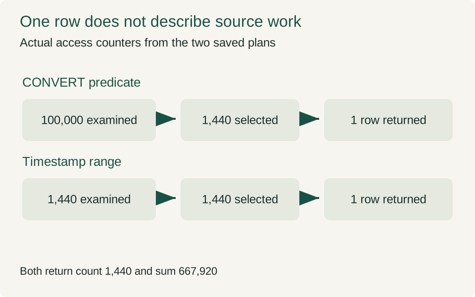
The middle count describes qualifying events and the last count describes result shape. The first count is needed to see the avoided access work.
Interpretation and evidence
- Read is not returned.
- One row can hide a scan.
- Validate the aggregate independently.
The actual plan for the conversion predicate contains a clustered index scan. Its runtime counters show 100,000 rows read and 1,440 rows produced by that access operator. The aggregate then produces the one result row returned to the client.
These are three different counts. Rows read describe what the access method examined. Rows produced describe what survived its predicate. Rows returned describe the final shape of the query result. Collapsing them into a single number makes the expensive part disappear from the explanation.
The range query's access operator is an index seek. It reports 1,440 rows read and 1,440 rows produced. The aggregate still returns one row with exactly the same count and sum as the conversion query.
The useful comparison is therefore not one output row versus another output row. It is 100,000 examined source rows versus 1,440, while preserving the same selected set in this fixture. That difference is visible before interpreting a stopwatch result.
Not every operator in the XML has a runtime counter block. The summary treats absent counters as unreported rather than manufacturing zero work. In particular, a compute-scalar node without its own reported runtime count should not be described as proof that scalar evaluation never happened.
The final row is still important. It is the acceptance boundary. The intermediate counts explain the mechanism used to reach it. Good diagnosis needs both: a correct result without work accounting can hide waste, while attractive operator counts with the wrong result are not an optimization.
The plan is not a literal drawing of the SQL text
03 / See the idea
The physical plan is not the SQL syntax
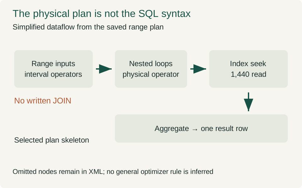
A nested-loops node appears in the actual one-table plan. It is an implementation choice here, not proof that an unintended relational join was added.
Interpretation and evidence
- Inspect operator responsibility.
- Do not diagnose by name alone.
- Keep the complete XML available.
The range plan includes interval-building operators and a nested-loops operator even though the SQL statement references only one table and contains no written JOIN. Its index seek consumes the resulting range and reads the 1,440 matching rows.
That observation is a useful reminder that physical operators are implementation choices, not one-to-one translations of keywords. Seeing nested loops does not establish an accidental relational join, just as seeing a sort would not by itself establish a bug.
The article does not attempt to generalize the optimizer's interval construction from this one plan. The saved XML is evidence of what this engine produced for these types and parameters. Explaining every future variant would require additional experiments and source-specific documentation.
The same caution applies to a common debugging instinct: removing DISTINCT because it looks expensive, replacing every nested loop with a hash join, or rejecting any scan. Such interventions can change the meaning of a query or worsen its plan under another distribution.
If the requested result genuinely requires duplicate elimination, that work belongs to the query's contract. If a scan reads nearly every row that must be returned anyway, a seek with repeated lookups may not be preferable. The appropriate question is which work is necessary for the intended result under the actual workload.
Our example keeps that question tractable. A selective daily interval exists in an ordered covered index, and both variants must return the same aggregate. The evidence supports discussing the avoided scan here without turning one successful rewrite into a universal style rule.
Estimates and actual counts answer different questions
The conversion predicate's scan estimates 10,000 rows but produces 1,440. The range seek estimates approximately 1,440.96 and produces 1,440. Those differences are useful observations, but they should not be overinterpreted.
The optimizer uses estimates to choose a plan before seeing the complete result. Runtime counters describe the execution that actually occurred. A close estimate can support a good choice, yet it does not prove the whole plan is ideal. A poor estimate can matter greatly in some queries and have little practical effect in others.
This experiment changes the predicate representation, which changes both the available access opportunity and the information used for estimation. It does not isolate estimate accuracy as the sole cause of the observed difference. Claiming that the query became faster only because the estimate improved would require another experiment.
Similarly, we do not infer memory-grant pressure or a spill from the estimate difference. Those mechanisms require their own evidence. The selected query is deliberately small in shape, and the captured access work is already sufficient to explain why final output size was a weak proxy for cost.
A useful investigation records estimates and actuals together, then asks which discrepancy could change the next decision. Collecting every plan property without a hypothesis can produce a large report while leaving the important mechanism unexplained.
Logical reads keep a warm scan visible
04 / Watch the mechanism
Follow a bounded range to its result
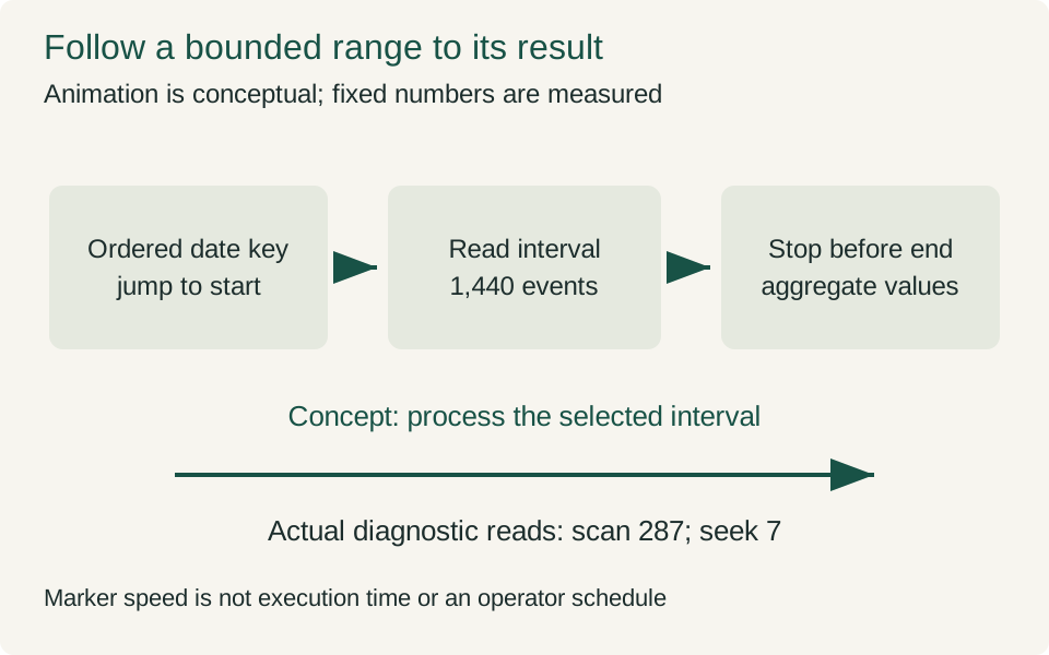
Static view. Play to see how the mechanism unfolds.
The animation shows the intended range restriction before aggregation. Its speed has no relationship to measured execution time, and all key information remains in the static poster.
Interpretation and evidence
- Restriction changes source work.
- Cached page reads still count.
- Motion explains dependency only.
STATISTICS IO reports 287 logical reads for the conversion query and seven for the range query. Both diagnostic executions report zero physical reads. That does not make the first query free; it means the page accesses were served without physical reads in those observations.
Microsoft defines logical reads as page reads from the data cache. They are distinct from physical disk reads, read-ahead activity and LOB accesses. These categories should not be added or relabelled casually. Microsoft: SET STATISTICS IO
The page count is not a guaranteed measure of unique pages, and it is not a network-byte counter. A page can be visited as part of execution work even when the final result contains only two scalar values. That is exactly why logical reads are useful in this example.
The diagnostic query uses STATISTICS XML to obtain an actual execution plan. This setting executes the statement and returns execution information, including runtime details. It has an observation cost, so the dedicated timing run does not enable it. Microsoft: SET STATISTICS XML
Keeping diagnostic and timed runs separate does not make them unrelated. They use the same schema, data generation, query text, parameter values and degree-of-parallelism setting. The evidence pack records those inputs so the reader can see which claim comes from which observation.
The narrower conclusion is strong enough: the range form used a covered seek and fewer logical page reads for the same result in this fixture. No assertion about disk throughput or production latency is needed to make that finding useful.
A result table needs its experimental boundary
05 / A concrete example
Same aggregate, different command time
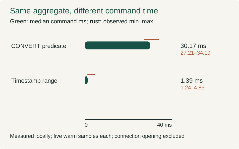
Green bars show medians of five samples per command. Rust lines and labels preserve the observed ranges; they are not confidence intervals.
Interpretation and evidence
- Five samples per command.
- Read range as observed variation.
- Apply only within this fixture.
The dedicated timing run warms the query shapes, then repeats them in five rounds with alternating order. Each date query therefore has five measured command executions in one prepared container environment. This is a small local experiment, not a population study of SQL Server performance.
The container is limited to two CPUs and 4 GiB of memory. Each query explicitly uses MAXDOP 1. The client and server communicate through an ephemeral port bound to loopback. Startup, schema creation, data loading and statistics update are outside the timer.
The measured interval starts before ExecuteReaderAsync and ends after the aggregate result is consumed. Connection opening is outside the interval. These choices make the command comparison repeatable but do not describe the full response time of a web endpoint, which could include authentication, connection acquisition and serialization.
The five recorded executions per query produced the following results. Every execution returned count 1,440 and sum 667,920. The logical reads come from the separate diagnostic executions, not from a counter sampled inside each timing interval.
| Query | Median ms | Observed range ms | Client allocated bytes, each sample | Diagnostic logical reads |
|---|---|---|---|---|
| Timestamp converted to text | 30.17 | 27.21–34.19 | 4,048 | 287 |
| Half-open timestamp range | 1.39 | 1.24–4.86 | 4,048 | 7 |
The recorded range-query times are 4.8552, 1.2419, 1.3933, 1.5103 and 1.3084 milliseconds. The first observation is visibly higher than the other four. It remains part of the evidence rather than being deleted as an inconvenient outlier. Five executions on a shared machine do not establish a service-level percentile or a stable production latency distribution.
The conversion-query times range from 27.2135 to 34.1944 milliseconds. In this small experiment, the ranges do not overlap. That supports a local command-time improvement alongside the stronger mechanism evidence: the range plan examined fewer source rows and requested fewer cached pages. It does not tell us how much faster an entire application becomes.
The identical client allocations are especially instructive. Both paths materialize the same tiny aggregate result, so that counter does not distinguish the amount of work performed inside SQL Server. An application allocation profile alone could miss this optimization opportunity completely.
Nor do the results prove a general cost per examined row. Parsing the predicate, traversing an index, evaluating expressions, aggregating values and transporting the response have different costs. Dividing elapsed time by rows read would combine those responsibilities into a misleading universal constant.
The timing result is interpreted after correctness and plan evidence. A smaller elapsed time with a wrong date boundary would be a failed comparison. A small or noisy timing difference would not erase the actual-plan observation; it would limit what we could say about user-visible benefit in this environment.
This ordering protects the investigation from a familiar trap. The chart should illustrate a mechanism supported by evidence, not become the reason to invent a mechanism after selecting an attractive number.
Change the workload before generalizing the rewrite
The generated timestamps are regular and the selected day is relatively selective. A real event table may contain bursts, retention gaps, hot partitions or a much wider result shape. Those conditions can change the best plan.
The next useful experiment depends on the intended deployment. If users select a month instead of a day, vary the interval width. If the query returns complete event records, remove the assumption that the index covers the result. If the table is under heavy writes, include the cost of maintaining the date index and the contention created by concurrent activity.
Do not change all those conditions at once and expect a clean explanation. Start with the uncertainty that controls the decision. The point is not to maximize the size of the benchmark matrix; it is to find where the current conclusion stops applying.
Parameter behavior also deserves its own study when workloads vary substantially. The plan for one day may not be suitable for another range. This article records one parameterized case and does not claim to solve parameter-sensitive planning for a production service.
The date definition must remain explicit throughout. A local business day crossing a daylight-saving transition cannot automatically be represented by adding twenty-four hours to a UTC boundary. This fixture avoids that question by using a declared UTC convention. A deployment with local calendar rules must establish its own interval semantics before borrowing the predicate.
Reproduce the question before reproducing the stopwatch
The code bundle contains the schema, deterministic data generator, C# collector and disposable-container wrapper. Reproduction begins with those inputs rather than with copying the table into a slide. The SQL Server image is pinned by digest, and the environment record captures the engine build actually returned by the server.
The client project pins its SDK, target runtime and package dependency. Those choices do not make every future host identical, but they remove an avoidable ambiguity about which client was used. The server compatibility level is 160 and both date statements include MAXDOP 1. A reproduction that changes either setting should record that difference rather than silently merging its results with this run.
The independent expected result comes from the fixture's arithmetic. There is one event per minute. The chosen interval contains exactly 1,440 such instants. The amount sequence follows a repeating integer rule, so the expected sum can be accumulated without querying the database. This is stronger than comparing two SQL statements that might share the same mistaken boundary.
For a new dataset, that oracle must be reconsidered. A timestamp can be missing, duplicated or recorded with another precision. The laboratory's arithmetic does not prove that a real event stream contains one row per minute. The reproducible part is the method of defining an independent expectation, not the accidental numerical answer.
The check command saves actual plans and diagnostic messages before the separate measurement command is used. Inspect the access operators first. Confirm their object names, actual rows read and output counts. Then locate the aggregate and confirm that its one row is the same result checked by the client. The saved plans are the evidence; the diagrams are simplified explanations of selected properties.
The measurement command prepares a fresh container and database, warms all six query shapes in the shared fixture, and records five alternating-order rounds. The JSON experiments include rolled-back updates to separate catalog tables. They do not modify Events, but they are part of the shared process history and can influence cache or host scheduling. This is another reason to describe the result as a controlled local comparison rather than an isolated engine microbenchmark.
When the run finishes, the wrapper removes its own container in a finally block. It uses an ephemeral loopback port, does not mount a persistent data volume and does not save its generated password. Cleanup is an actual recorded outcome of this execution. The evidence pack preserves the query inputs, results and plans needed for review without preserving a database service that the next reader might accidentally reuse.
If a reproduction yields a different plan, that is a useful observation to investigate. Verify the schema and parameters, compare the actual server build and compatibility level, and examine estimates and row counts. Do not force the original plan merely to make the chart agree. The purpose of the laboratory is to make the mechanism inspectable, including the conditions under which it changes.
Use the final row as a contract, not a cost estimate
The client received one row in both cases. That row was necessary to establish correctness, but almost useless as a description of how much source data the engine examined.
The actual plans supplied the missing distinction: a scan reading 100,000 rows versus a seek reading 1,440, both feeding the same one-row aggregate. Logical reads supplied another perspective on the avoided work. Timings then described the local cost of executing those paths under the recorded conditions.
This method scales beyond date predicates. A report can hide a multiplied join result beneath an aggregate. A DISTINCT can conceal either a legitimate requirement or an incorrect relationship. A small API response can be the last step of a much larger computation.
The disciplined response is to preserve the meaning of the requested result, inspect the actual intermediate work and choose a change whose effect can be tested. It is neither to trust every compact query nor to reject every complicated-looking plan.
The next time an application returns a single reassuring number, ask how many rows had to be read, filtered, joined or aggregated to produce it. Then ask which of that work the result actually requires. Those questions begin a performance investigation that the response size alone cannot answer.
Source code and execution evidence
Download the complete lab, source record and raw execution results. This package supports the specific execution claims in this article. It is not a production certification.