

Series How .NET Runs Your Code, part 9 of 11. Previous: Part 8, startup and the first correct response. Next: Part 10, working set, heap and retention.
Dana has opened the first correct partner file from Intake's Native AOT worker. It uses the explicit XML writer that replaced the failed reflection-based exporter in part 1. Now the fictional team needs to choose a build for a busy queue. If two workers deliver the same number of correct files each second, can Ravi expect the same CPU use per delivery? Can Dana promise customers the same wait?
The ordinary build uses a just-in-time compiler (JIT). Native ahead-of-time compilation (Native AOT) puts machine code in the artifact. Lena has a second question. If she keeps the ordinary build and upgrades the API from .NET 10 to .NET 11, will more customers meet their deadline?
- For the API, count a verified acknowledgement for the submitted name. For the worker, count the partner file after its XML has been parsed and checked.
- Use elapsed time for throughput, process CPU time for CPU cost per correct job, and each job's enqueue and completion timestamps for latency. For independently scheduled arrivals, include the wait to send.
- On the same Windows x64 machine, one Native AOT publish option changed the pool that served a verified request. A separate Windows trial changed the ordinary API’s runtime and kept its publication strategy fixed.
- A faster temperature scan in memory did not yield a repeatable gain for the complete CSV import on any of the three machines. Counting while parsing saved memory on all three.
Count the job that the client can identify
The ordinary .NET 11 API on the Arm64 Mac received three named submissions with up to two in flight. The client numbered its inputs before the server assigned job IDs. Predict whether rebuild-index-1 got ID 1, then read the three rows in the order the client recorded them.
input,verified_id
rebuild-index-2,1
rebuild-index-1,2
rebuild-index-3,3
The second input got the first ID. A test that equates the launch sequence with the server's assignment would reject valid work under concurrency. The client instead checked HTTP 202, the location /jobs, the exact name, and a positive integer ID unique in this process. A separate GET /jobs recovered the same three name/ID pairs and a count of three.
The worker has a different finish line. It reads one named job per line, evaluates the configured rule and writes a bounded XML export into a fresh directory. The client must match the worker's acknowledgement to the right document, parse it and read back the job name. What would a green acknowledgement hide if the writer produced the wrong file?
The worker earns a completion when the partner can read the submitted name
- The client issues a specific job name. Its pending slot stays occupied while the worker evaluates the policy and creates the document.
- The bounded writer escapes the job name and makes the completed file available to the independent consumer.
- The acknowledgement associates the submission with the next worker output. Reading that line is only the first half of the client's check.
- The consumer opens the matching file and parses its root and child. An unexpected shape or name fails the operation.
- Once the checked file is consumed, the client records a completion and makes its slot available for the next job.
Operation from bench/harness/load.py using the 1,024-byte fixture. The fixed-work receiver records are in results/mac/part09 and the matching Windows and Linux folders.
Worker replies carry no ID, so the client serializes the writes to standard input and keeps the corresponding names in a first-in, first-out queue. A leftover partner file also fails the trial. This trial covers the partner-directory workload. A worker deployment that also polls the API journal has an additional network and storage path.
The same checks ran for both .NET 10 and .NET 11. The candidates included ordinary JIT builds, ReadyToRun builds with precompiled managed code, native builds and their single-setting controls. In total, macOS Arm64 verified 96 jobs in 32 fresh processes, Windows x64 verified 108 in 36, and native Linux x64 verified 96 in 32. Windows includes the extra portable-pool variants. Each launch performed exactly three operations. These counts establish which candidates can enter a capacity comparison.
Three measures start from the same verified jobs
Keep the jobs that finished in a chosen interval. For throughput, divide their count by elapsed seconds. For CPU cost, divide the target process's CPU-time increase by that same count. For latency, retain each finished job's time from client enqueue to verified result and report the distribution of those waits. For the 99th percentile (p99), the driver sorts the waits and takes the observation at rank ceil(0.99 × n), counting from one. A process can spend CPU on work still in flight at the cutoff, so the cost ratio belongs to the whole window. It does not assign processor time to an individual request. What TotalProcessorTime counts.
The example below uses manually specified values from the download's reporting test. Each of the last two one-second windows contains two finished jobs and 1 ms of process CPU. Select seconds three and four in turn. Which reading changes even though the completion count, elapsed time and CPU charge all stay fixed?
Equal throughput and CPU cost can hide a change in customer latency
- The process consumes CPU before the first verified reply arrives. Throughput is zero, and dividing the CPU charge among zero completed jobs has no defined result.
- One job finishes. The process used one millisecond of CPU in this window, while the client recorded twenty milliseconds between enqueue and verification.
- The aggregate CPU charge is half a millisecond per completion. The two individual waits are two and five milliseconds, so the nearest-rank p99 selects five.
- The same number of jobs finish for the same CPU charge. The recorded waits are now seven and nine milliseconds. Rate and CPU cost alone miss the change.
- Pool the four completed waits before taking the percentile. The combined median is six milliseconds and p99 is nine. Four observations offer little resolution in the tail.
Illustrative arithmetic from the fixed inputs in bench/harness/test_load.py, test test_startup_zeroes_and_cpu_cost_are_charged_to_their_own_windows. Each one-second window accrues 1 ms of process CPU. No Intake timing samples appear in the figure.
There is a second trap in the pooled window. Averaging the two p99 values would give (5 + 9) / 2 = 7 ms. Ranking the four original waits gives 9 ms. Keep the individual waits or a mergeable histogram. The three fixed-work receivers supplied correct outputs without elapsed durations. What can their binaries tell Lena about the work to measure next?
The same interface call has several possible machine-code bodies
Take one part of that work out of the queue. RuleLoop.CountAllowed receives an IPayloadRule and four payload sizes: 0, 1,023, 1,024 and 1,025 bytes. It counts the values the rule allows. The production worker applies the same interface to individual jobs. The diagnostic driver isolates the helper, letting us open its instructions without confusing rule evaluation with file I/O.
Two implementations are reachable in the diagnostic executable. The usual PayloadRule accepts equality at the 1,024-byte limit. StrictLimit performs a direct less-than comparison and rejects equality. The caller chooses one at startup. In each finite run the helper was called 327,680 times. Three accepted inputs per inclusive call give 983,040. Two per strict call give 655,360. Both publishing modes returned their respective expected totals. The pauses between batches give the ordinary runtime opportunities to promote code. Reaching Tier1 for this helper establishes a compilation event. A service-wide plateau would need a separate series of completed jobs and CPU readings.
Now follow Allows inside the ordinary .NET 11 Mac process. Its dynamic profile-guided optimization (PGO) can use observations from earlier calls when it compiles a method again. In quick code the runtime dispatches through the interface, which means finding the right method for the object currently passed. The caller repeatedly supplies the inclusive implementation in this run. Before viewing the later body, predict which part can be inlined and what must happen if a different object arrives.
The JIT keeps an interface fallback and the native loop contains two known paths
; Assembly listing for method Intake.Rules.RuleLoop:CountAllowed(Intake.Rules.IPayloadRule,int[]):int (Instrumented Tier0)
blr     xip0      // code for Intake.Rules.IPayloadRule:Allows(int):bool:this
; Total bytes of code 316

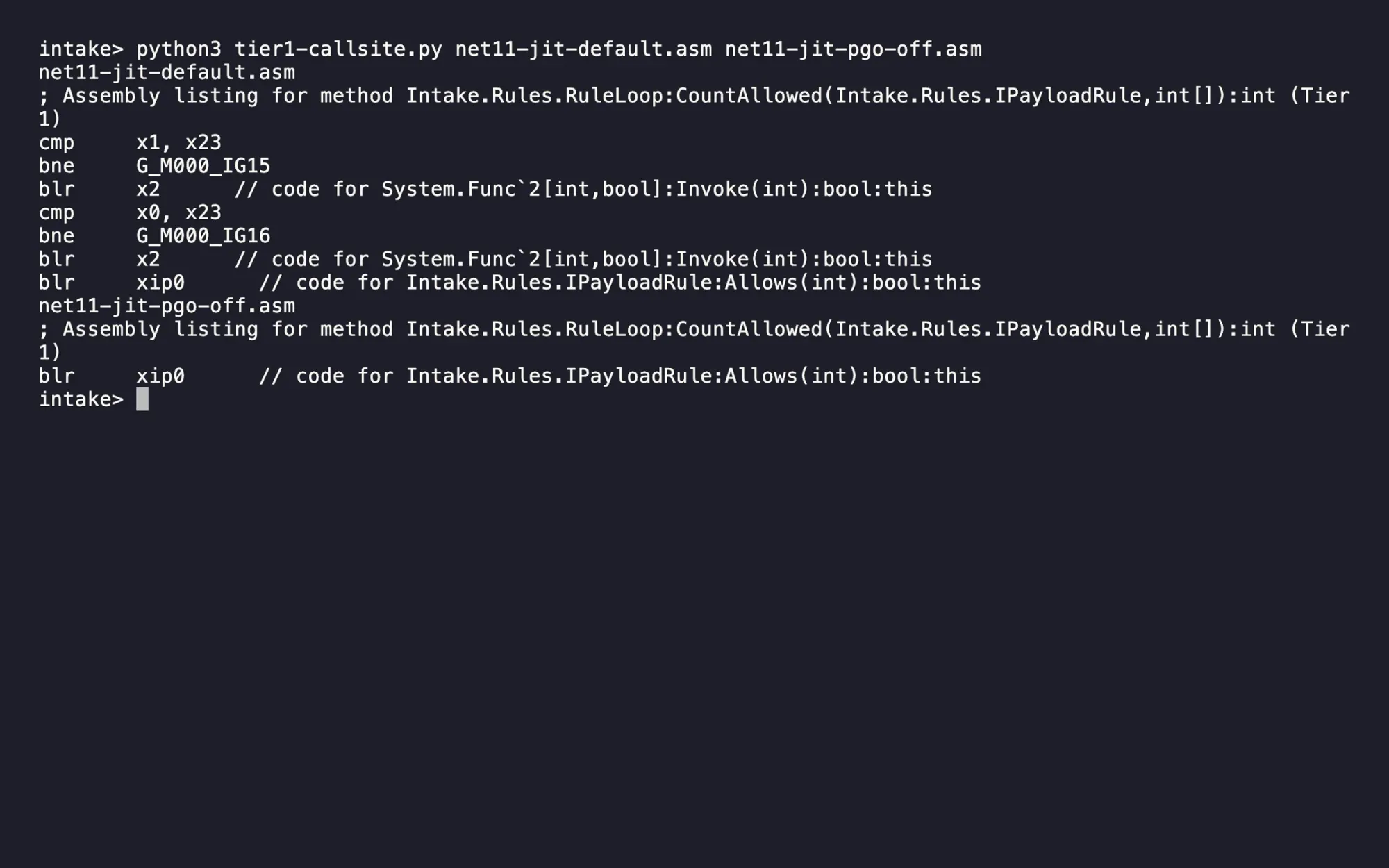
; Assembly listing for method Intake.Rules.RuleLoop:CountAllowed(Intake.Rules.IPayloadRule,int[]):int (Tier1)
cmp     x0, x23
bne     G_M000_IG16
blr     x2      // code for System.Func`2[int,bool]:Invoke(int):bool:this
G_M000_IG16:
blr     xip0      // code for Intake.Rules.IPayloadRule:Allows(int):bool:this
; Total bytes of code 228

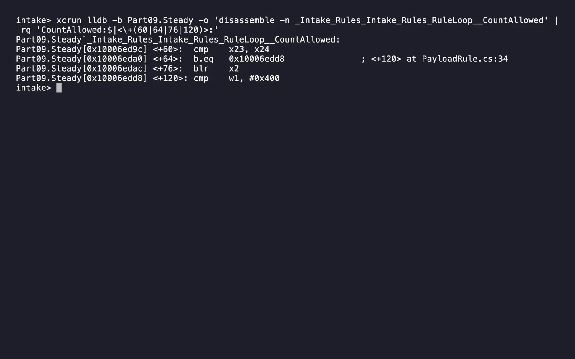
; Native file, same method
cmp    x23, x24
b.eq   0x10006edd8
ldp    x0, x2, [x2, #0x10]
blr    x2
Part09.Steady[0x10006edd8] <+120>: cmp    w1, #0x400
b.ge 0x10006edb8- The instrumented first version dispatches through IPayloadRule.Allows. This excerpt omits loop bookkeeping and the calls used to collect profile information.
- The later JIT body checks the receiver type. On a match it reaches a delegate invocation inside the inlined wrapper.
- The fallback block still has an interface call. A receiver missing from the observed profile must be able to produce its own correct decision.
- The native file also compares a type pointer. On one path the instructions load a delegate target and invoke it indirectly.
- The other native branch compares the payload with hexadecimal 400, the strict limit. The alternate runtime input exercises the equality difference.
Filtered JIT and AOT listings from results/mac/part09/code on Arm64. The excerpts retain the branch targets and omit setup, loop bookkeeping and epilogues.
The blr on the matching JIT path still invokes a delegate. Knowing the wrapper type has eliminated one level of indirection, while execution of the customer's expression remains a separate call. The type check and the fallback together make this guarded devirtualization. The runtime team's explanation of profiled dispatch.
Open the Native AOT executable in a debugger. Without a live profile, must the compiler dispatch indirectly? The Arm64 file compares the method-table pointer with a known type. One branch calls the delegate. The other compares the payload with 0x400 (1,024) and rejects values at or above the limit. That branch implements the strict rule. The compiler knew which implementations were reachable before the first customer arrived.
A third reachable rule could change the native compiler's choices. A different customer mix could change the ordinary runtime's profile. To see whether dynamic feedback matters at this site, keep the executable and repeated inputs fixed and switch off just that feedback.
Turning off dynamic PGO changes the code you are comparing
To isolate dynamic PGO from tiered compilation itself, keep the executable fixed and run it again with DOTNET_TieredPGO=0. A third process uses DOTNET_TieredCompilation=0. The same inclusive rule and inputs must still return the same count. Look at the final listing header as well as the body size.
| .NET 11, Mac Arm64 | First observed body | Last observed body | What the loop contains |
|---|---|---|---|
| Default | Instrumented Tier0, 316 B | Tier1, 228 B | A guarded delegate path and an interface fallback |
| Dynamic PGO off | Tier0, 232 B | Tier1, 120 B | An interface call remains |
| Tiering off | FullOpts, 120 B | Same single body | Full optimization on first compilation |
The PGO-off process still reached Tier1. Its 120-byte body keeps the interface call. The default process spends more bytes on a guarded path. A useful next experiment keeps the same rule mix on both sides and compares the CPU cost of correct results.
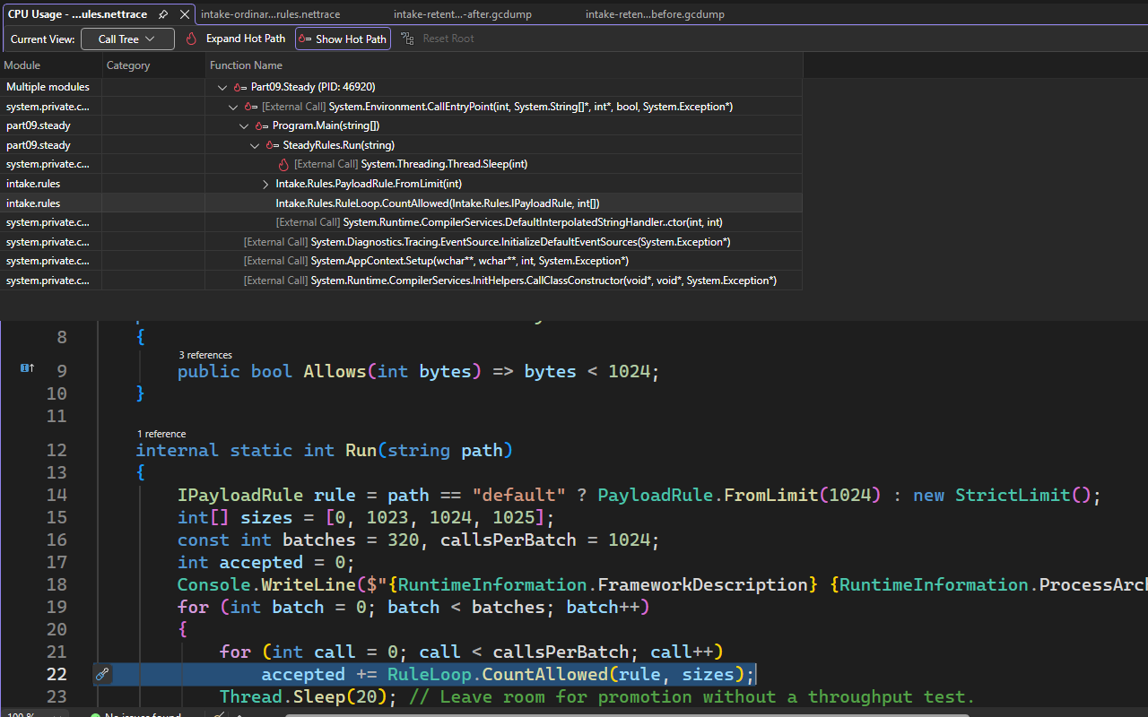
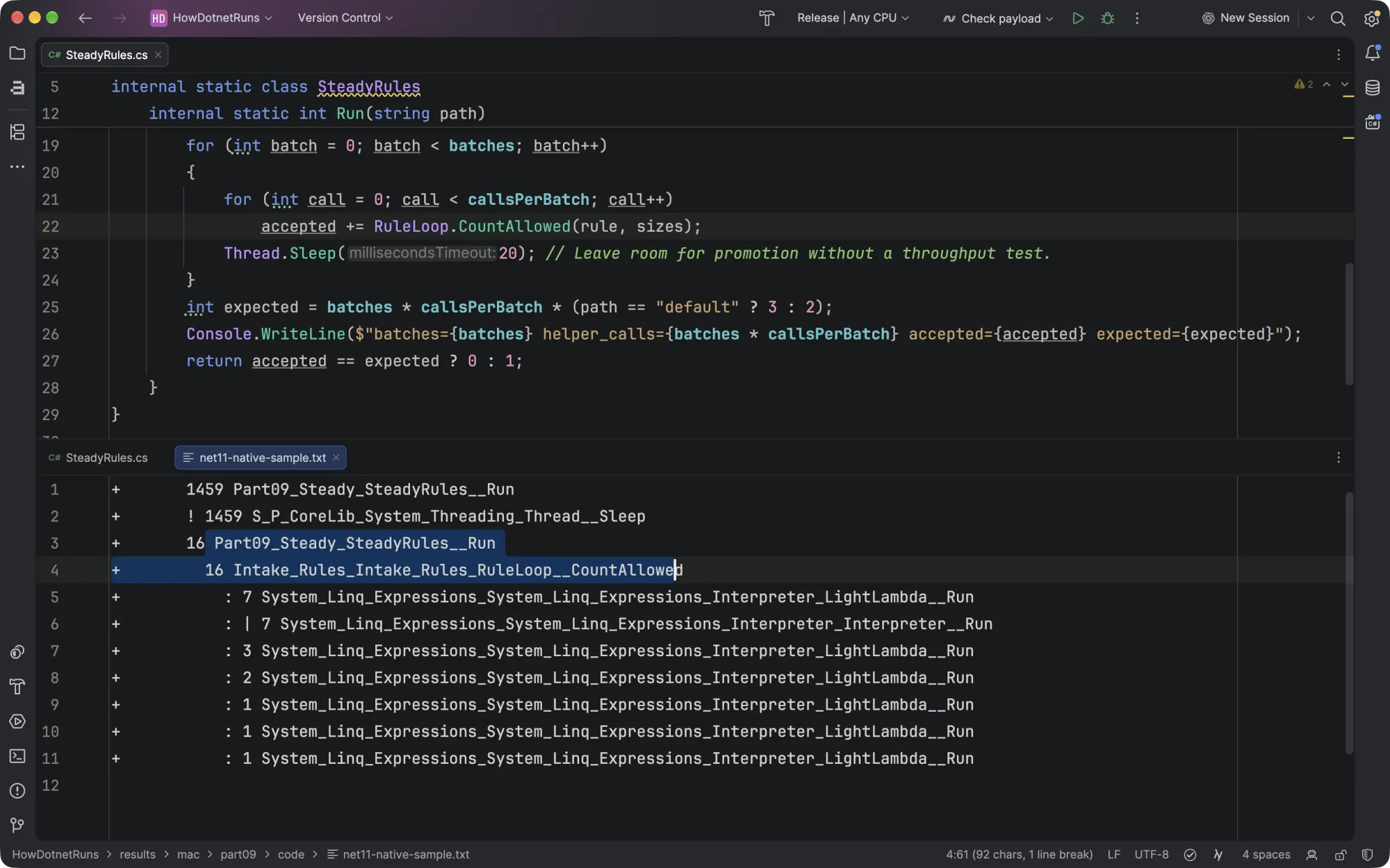
A sampling trace gives a different view. In the Windows JIT trace, the CPU Usage call tree ties SteadyRules.Run to Intake.Rules.RuleLoop.CountAllowed. In the native Mac process, an external sampler caught RuleLoop.CountAllowed above LightLambda.Run and the expression interpreter. Part 5 showed why the default expression delegate takes that route on Native AOT. Matching a JIT call and a native call at the interface does not guarantee that the work behind the interface is identical. Before blaming the dispatch, try the strict source-written rule on both sides, and keep its different equality contract explicit.
A speed hint and a CPU target produce different binaries
Ravi can also give the ahead-of-time compiler more information. OptimizationPreference=Speed changes its trade-off between code size and execution speed. In these runtime packs it also enables the build logic that can supply the framework's static profile files, where available. Those profiles were generated ahead of time. They contain no observations of Intake's customers on this particular receiver. Native AOT optimization options and the SDK's Native AOT targets.
A different build uses IlcInstructionSet=native, asking the compiler to target the build machine's processor capabilities. The file passed on its build receiver. Qualify it on each CPU baseline in the deployment, as in part 7.
These are the individual options selected by the sample's native variant driver. The Windows-only pool option is a third candidate. Build each with the same registered API contracts, bounded XML exporter, runtime and target. On Windows the command below selects all three .NET 11 variants by default. It writes a per-file inventory and verifies the published API and worker for each one.
py -3 tools/part09.py tuned --work native-files --out native-resultsOn AMD Windows x64, the .NET 11 default native API executable was 10,832,384 bytes and the worker was 9,119,232 bytes. Which setting added most to each executable?
The Speed candidate added the most executable bytes on this Windows host
| Changed option | API | Worker |
|---|---|---|
| Speed | 520.5 | 402.5 |
| Host instruction set | 32.5 | 24 |
| Portable pool | 50.5 | 58 |
- Each bar compares one Windows x64 API executable with the same runtime's native default. The effect shown is the change in file length.
- The bounded XML worker has different reachable code. The same compiler settings therefore produced different size changes for its executable.
- The portable-pool build brings a different scheduler into the file. Its live identity is checked on a separate instrumented pair.
Derived from executable bytes in results/win/part09/images.tsv on AMD EPYC 7502P. One KiB is 1,024 bytes. Debug symbols are excluded.
Watch what happens if a build report compares entire directories instead. The Speed build increased the Windows API executable by 532,992 bytes. Its full publish folder, including symbols, went from 57,457,945 to 57,147,161 bytes. The debug-symbol PDB shrank by 843,776 bytes. If symbols ship separately, count the executable and symbol archive separately too.
On the Mac, the default and host-ISA .NET 11 native API executables both measured 9,873,288 bytes and had different SHA-256 hashes. Equal lengths establish neither identical contents nor a performance tie. On Linux x64, the same setting moved the API executable from 10,194,808 to 10,227,608 bytes. The toolchain and target decide what ends up in each file. A run on one matching processor does not establish how much CPU that change saves in service.
Which thread pool served the request?
An ordinary Windows build normally uses the portable .NET pool. Native AOT on Windows delegates worker management to the Windows thread pool by default. Keep the same AMD EPYC receiver, Windows kernel and native build settings, then change one publish property, UseWindowsThreadPool. Which pool actually handles the request? Windows thread-pool selection.
Two instrumented Windows x64 API builds observed hosting event 3, RequestStart, on a real POST /jobs. The listener also queued one callback. The client verified the returned job name and ID against the journal. Look at the thread-entry frame in each request stack, shown here for .NET 11.
Microsoft.AspNetCore.Hosting event=3 POST /jobs
at System.Threading.WindowsThreadPool.DispatchCallback(IntPtr, IntPtr, IntPtr)

Microsoft.AspNetCore.Hosting event=3 POST /jobs
at System.Threading.PortableThreadPool.WorkerThread.WorkerDoWork(PortableThreadPool)
at System.Threading.PortableThreadPool.WorkerThread.WorkerThreadStart()
The default build took the first path. Publishing with UseWindowsThreadPool=false gave the second. The queued callback matched the request’s pool on both .NET 10 and .NET 11. Both Windows builds reported server GC.
A deployment ticket proposes moving the API to Linux to fix a tail-latency problem. Windows and Linux share an AMD host in this study. Is keeping the processor enough to isolate the thread pool? Follow one row at a time and identify what changed.
Only the Windows pair changes one pool setting on the same machine
On a narrow screen, swipe left or use the right arrow key to see what each pair establishes. Windows request and callback stacks come from the Part 9 pool records. Linux supplied name/ID checks. The Part 10 heap reports identify the ordinary Windows and Mac pool type.
In part 10, the .NET 11 append experiment found one System.Threading.PortableThreadPool object in each ordinary Windows and Mac baseline heap. A separate .NET 10 Mac dump names PortableThreadPool+WorkerThread.WorkerThreadStart() on a thread. Neither record ties that thread to a particular HTTP request. For each native Linux x64 build, the client verified three named API responses and the journal. The Unix runtime uses the portable pool, but these Linux records contain no request stack. Unix thread-pool implementation.
To test the ticket, repeat identical arrivals on the two uninstrumented Windows builds. If the portable build meets the deadline, Dana already has a Windows candidate. Compare Linux as a separate deployment under matched resource limits. The ordinary API in the next clip illustrates the limitation of a live queue counter. A zero reading cannot reconstruct a customer’s earlier wait.
The slowest request needs a start point as well as a finish point
For an API caller, the wait ends at a correct response. For Intake's partner, it ends at a readable XML document. Start the clock at the client. A handler timer misses queuing and connection setup. The publish-mode harness opens a new loopback connection per operation. A production client with persistent connections needs its own trial.
Each slot in Intake's closed-loop client stays occupied until its request completes. During a stall, the next submission waits for a free slot. The CSV records customer waits for submitted requests, but the jobs an independent producer would have sent leave no rows. The runtime migration trial below schedules these arrivals independently. How open and closed arrival models differ.
The driver bins a success by completion time and keeps the start offset. A request enqueued during warm-up can contribute its entire wait to a later window. Jobs drained after the cutoff are counted separately.
A five-second test after launch
Start both processes on the same cores and count responses for five seconds. Startup consumes part of the window, the client competes for CPU, and a 202 can identify the wrong job.
Five independent rounds with the same completion test
Run verify against the published files. On a quiet receiver, reserve distinct CPU sets. Keep warm-up and verified operation rows. Compare post-warm-up rate, CPU per result and the latency distribution against the release budget.
Separate elapsed seconds from CPU-seconds
Start sampling before launch. Keep the first 60 seconds as ramp and the next 60 as a candidate steady window. Preserve empty early seconds. If the later rate is still changing, retain that series and run a longer trial.
The observer reads TotalProcessorTime from the single server or worker process that it owns. A CPU cost of c positive milliseconds per verified job corresponds to 1,000 / c jobs per CPU-second. Throughput divides completed jobs by wall-clock seconds instead. If XML writing or validation moves into a separate helper process, the original PID's counter no longer covers the same work.
Put executable paths, runtime, target and CPU assignments in cells.json. On quiet Linux or Windows, publish the observer, supply a receiver-specific lock and use a fresh output directory. The functional command also runs on macOS.
python3 -B bench/harness/load.py verify --manifest cells.json --concurrency 2 --out checked-jobs
dotnet publish src/Part09.Steady -c Release -o observer
python3 -B bench/harness/load.py measure --manifest cells.json --shape api \
  --concurrency 4 --warmup 60 --seconds 120 --rounds 5 \
  --observer observer/Part09.Steady --quiet-receiver quiet-linux \
  --measure-lock .measure.lock --out receiver-api
Each round shuffles the candidates with a recorded seed and launches fresh processes. Inspect the per-second trend, sample counts and actual counter-read offsets before comparing rounds. Choosing the measurement that matches the service.
Will .NET 11 meet the API deadline as arrivals rise?
Lena keeps source and publish mode fixed. Both framework-dependent Release builds use the ordinary JIT. On a shared Windows Server 2022 host with an AMD EPYC 7502P, the API had four assigned cores and the loopback client two others. Background activity was recorded while Docker and WSL workloads stayed active.
Each fresh API process accepted 300 warm-up jobs before a ten-second step to a common offered rate. Increasing that rate also grows the journal faster. The HTTP/1.1 client kept connections open and capped outstanding requests at 32. A job counted only after the client read HTTP 202, Location: /jobs, the submitted name and a unique positive ID. A final GET /jobs checked those pairs against the journal. Where does a late dispatch appear in the customer’s wait?
The deadline clock starts at the scheduled arrival
The client keeps each scheduled slot. An unsent slot has a drop reason and empty send and finish timestamps. The arrows show event order.
In the first 12/s pair, request 53 shows where a long wait accumulated. On .NET 10 the client dispatched it 0.52 ms late, then waited another 771.0 ms through verification. On .NET 11 the same two intervals were 1.00 ms and 738.5 ms. The longer interval includes client, transport and server. Rank the complete waits (done_ns − scheduled_ns) to get p99. Adding the two component percentiles can combine different jobs.
At each offered rate the team ran six pairs of fresh processes, with each runtime going first three times. Read down the chart from scheduled p99 to dispatch delay. Each point summarizes the pairs that verified every scheduled job on both runtimes. The whiskers span the accepted block values.

What happened to customers in the excluded runs? The table includes all six runs per version and rate. Its p99 ranks all verified jobs together, including replies from excluded pairs. CPU per job divides the server’s CPU milliseconds through the final drain by its verified jobs. The journal read follows that window. For the last column, suppose the service-level objective (SLO) requires 99% of all offered jobs to return a correct 202 within 10 ms of their scheduled arrival.
| Offered/s, .NET | Verified / offered | Dropped | p99 (ms) | CPU ms/job | By 10 ms |
|---|---|---|---|---|---|
| 10 / 10.0.15 | 599 / 600 | 1 | 774.4 | 0.23 | 92.2% |
| 10 / 11.0.0 | 598 / 600 | 2 | 803.6 | 0.26 | 90.8% |
| 12 / 10.0.15 | 718 / 720 | 2 | 691.0 | 0.22 | 91.8% |
| 12 / 11.0.0 | 720 / 720 | 0 | 685.3 | 0.22 | 92.1% |
| 25 / 10.0.15 | 1,500 / 1,500 | 0 | 872.8 | 0.34 | 79.0% |
| 25 / 11.0.0 | 1,498 / 1,500 | 2 | 841.2 | 0.21 | 82.0% |
| 50 / 10.0.15 | 2,904 / 3,000 | 96 | 818.0 | 0.37 | 83.2% |
| 50 / 11.0.0 | 2,837 / 3,000 | 163 | 890.2 | 0.46 | 80.8% |
Both runtimes missed the example SLO at every offered rate when all six attempts were combined. At 50/s, 93 of the 96 drops on .NET 10 and 160 of 163 on .NET 11 hit the client’s 32-request limit. The other three on each runtime missed their dispatch slot. Every sent request returned a verified response. A successful-response p99 alone hides those unsent jobs. A separate 200/s pilot also lost scheduled arrivals, so neither result locates the API’s capacity limit.
CPU has limited resolution in these short windows. Across 100 completions at 10/s, a single observed 15.625 ms increment in process CPU changes the reported cost by about 0.16 ms per job. For a migration decision, repeat the paired trial with a generator that can maintain the intended arrivals, preserve the same deadline, and inspect both send and reply timestamps. The download keeps the individual requests under results/migration/cohorts/post-recovery-shared-host/runs/api/.
Choose the comparison before choosing a processor
On the same Arm64 Mac the profiled JIT helper went from 232 bytes on .NET 10 to 228 on .NET 11. On Windows x64 it went from 150 to 152. Each comparison varies the .NET line on a fixed receiver. The .NET 11 runtime also has a shared helper for surviving interface calls. The delegate invocation in our native listing does not identify that helper. .NET 11 Native AOT dispatch.
AMD versus Intel x64. Run the same OS image and x64 publish folder on two quiet receivers. Verify the whole folder fingerprint and use an instruction baseline supported by both CPUs. Rebuilding with IlcInstructionSet=native on each host answers a second question about separately tuned deployments.
x64 versus Arm64. Keep the Linux distribution, runtime release, source, build options and application inputs fixed. Publish for each architecture and record both hashes. Comparing Windows on the EPYC with macOS on the M3 Max instead evaluates two complete deployments. It cannot isolate instruction set, manufacturer or OS.
Match CPU allocation, memory limits, storage and client placement. Replay the same arrival schedule and job mix in repeated quiet rounds, with the load generator outside the target's cores. At the required throughput, both candidates must deliver the expected jobs and meet the agreed p99 deadline. A repeatable reduction in CPU per verified result, larger than the variation between rounds, identifies the more CPU-efficient deployment for that workload. For a purchase, compare billed cost per verified job as well. Intake’s worker still needs that service-level trial on Intel.
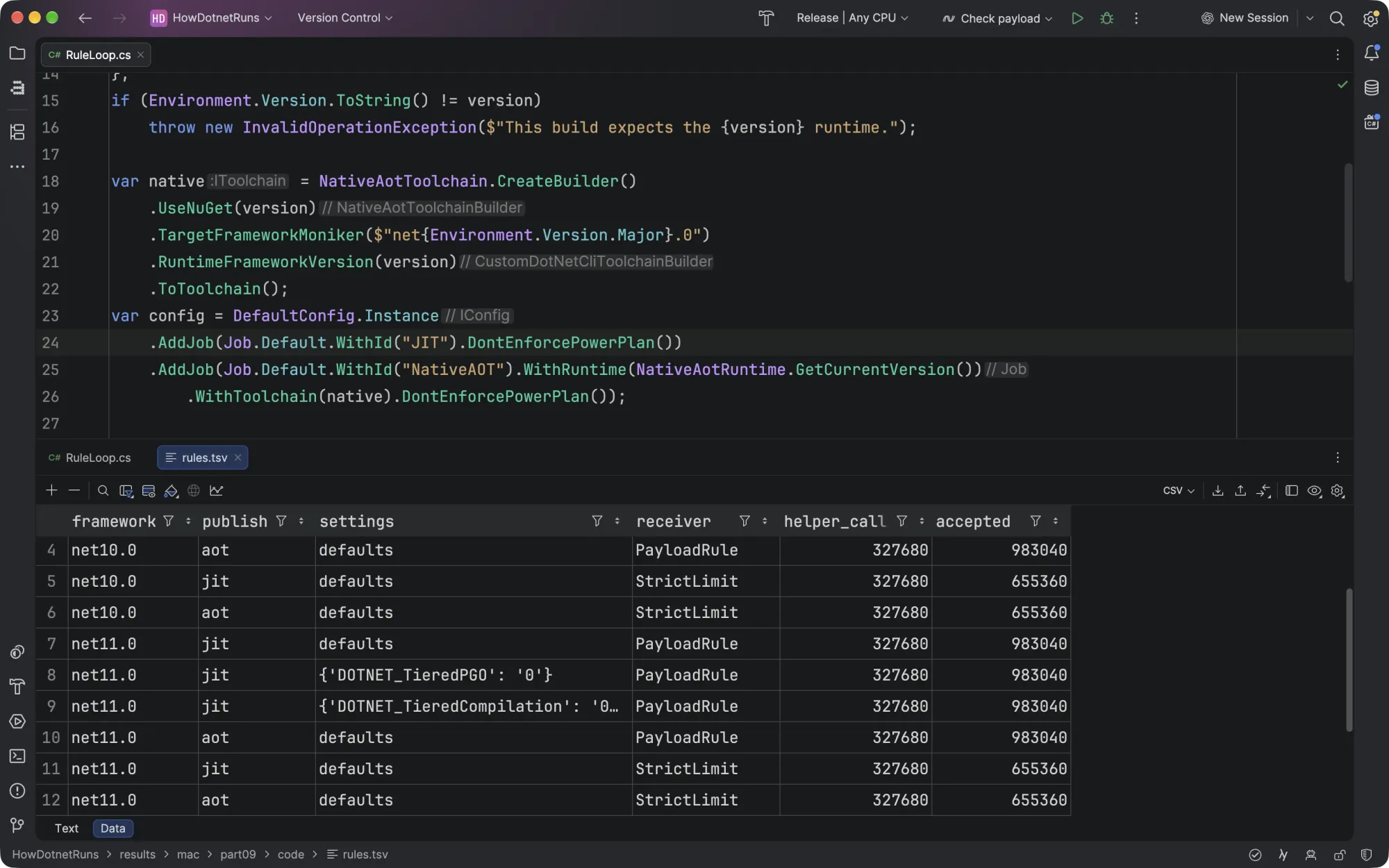
Use the microbenchmark to examine a mechanism after the service comparison points to it. Both BenchmarkDotNet jobs below call WorkerPolicy.CountAllowed on the same four inputs and leave the receiver's power plan unchanged. native selects the matching Native AOT compiler package.
var config = DefaultConfig.Instance
    .AddJob(Job.Default.WithId("JIT").DontEnforcePowerPlan())
    .AddJob(Job.Default.WithId("NativeAOT").WithRuntime(NativeAotRuntime.GetCurrentVersion())
        .WithToolchain(native).DontEnforcePowerPlan());
Benchmark discovery listed that method on both target runtimes. The table in the following capture comes from the separate fixed-work runs. The quiet-receiver benchmark jobs have no measured time result here.
Which machine scans an array of temperatures fastest?
Imagine importing a month of sensor readings and counting the readings above 85 °C. Once the temperatures are in an array, that count needs one pass. The same .NET 11 JIT program timed that pass on three machines, using one thread.
The first panel shows the widest implementation the sample could run on each machine. The second panel fixes the width at 128 bits. Read the 4,096-reading row in those two panels. The last panel shows the separate M3 confirmation. Which machine has the highest median in each? Part 2 shows the counting code and how to rerun it.

At 4,096 readings, the Xeon reached a median 21.1 billion readings/s at 512 bits. At a common 128 bits the EPYC reached 8.25 billion/s and the Xeon 7.45 billion/s. At 128 MiB the M3 Max had the shortest median scan time in the three-machine test. A separate M3 confirmation used 24 new processes across three sessions. Its 128-bit loop beat its own scalar loop in every pair at 37, 4,096, 1,048,576 and 33,554,432 readings. On the largest buffer the median paired speedup was 2.12×. The measurements describe one thread on these shared machines, with macOS, Windows and Ubuntu respectively. In the download, open results/temperature/report.html to change the buffer size and inspect the actual time for each supported implementation.
Does a faster counter finish the CSV import sooner?
Ravi receives a motor sensor export with one Celsius reading per line. He needs the count above 85.00 °C. A short file holds 37 readings in 252 bytes. At one reading per second, a full day gives him 86,400 rows. Our generated day file is 563,281 bytes. The first rows include 85.00, 84.99, 85.01 and -0.01. Only 85.01 should trigger an alarm. A separate decimal calculation gives Ravi two answers to check, 22 for the short file and 39,999 for the day.
Every timed import opens the file, reads its bytes, closes it and parses the decimal text. Two versions count line breaks to size an int[] and fill it with temperatures in hundredths of a degree. Only the final count changes. The scalar loop checks one integer at a time. The SIMD loop uses one instruction on several integers, choosing 128 bits on the M3 Max, 256 on the EPYC and 512 on the Xeon. Both versions use the same file and parser code. How File.ReadAllBytes opens and closes the file.
Each machine ran eight fresh .NET 11 processes. In each process, every version imported the file once before timing began for that file. The timed repetitions reopened it with the operating system’s file cache already warm. In each panel, compare the two bars on the same machine first. The short-file panel uses microseconds and the day panel uses milliseconds. Does the shorter bar also win consistently within individual processes?

On the EPYC the day-file medians look promising, 1.83 ms with scalar counting and 1.69 ms with SIMD. Pair the runs within each process and the median speed ratio is just 1.017, with four SIMD wins in eight pairs. The rule set before timing required a ratio of at least 1.05 and seven wins. SIMD cleared that bar for neither file on any of the three machines. For this importer Ravi can keep the simpler counter. A service that already holds parsed temperatures can use the array results above.
Ravi can make a different change if the alarm count is the only output. Increment it as the parser produces each temperature. This version skips the preliminary line count, the integer array and the later scan. It still reads the entire file into a byte buffer. For a day file it allocated about 338 KiB less managed memory per import on each host. That change also fell short of the timing rule on all three. Keep the parsed values when the next operation needs them. Part 10 traces the allocation difference to the arrays the importer creates.
To repeat the measurements, open bench/temperature/FileImport in the download and run the two commands below. The second command generates both files, verifies the counts and writes your eight process blocks. On Windows use py -3 for python3.
python3 -m zipfile -e ../import-kit.zip kit
python3 repeat.py kit/FileImport.dll my-import-run
Open TemperatureImport.cs to see where the three paths diverge. In the download, results/temperature-import/paired-blocks.csv gives the two times behind each win. A command-line tool that starts once per file also pays to launch the process. Part 8 measures that wait on the same two files. What happens if the next file arrives while that command is still starting?
Did the sensor publish 125 files per second, or did the worker finish that many?
Take the first dense arrival window on the Windows EPYC. The producer made 32 small files available over 247.6 ms. Across those 31 gaps, the observed arrival rate was 125.2 files/s. Ravi’s dashboard could show that number even if the importer stopped checking files altogether. How many files still lacked a checked alarm when the last one arrived?
With a fresh command per file, 27 of the 32 were still waiting for an answer. The final file ID and temperature count checked out 1,384.3 ms after the first release. Divide 32 by those 1.3843 seconds and the receiver delivered 23.1 checked alarms/s. In the corresponding run, starting a command immediately with up to eight already-ready files delivered 100.4 alarms/s, with six still awaiting an answer at the last arrival. Both policies used the same scalar importer. The producer ran on its own schedule in both runs.
Starting the clock too late also hides the slow alarms. Across all 128 EPYC files on the dense schedule, the per-file CLI had a p99 of 44.6 ms from dispatch. Starting at the actual release of each file brought its p99 to 1,094.8 ms. Open results/temperature-arrivals/explorer.html in the download and select a late file to see how long it had already waited before dispatch. Part 8 plots the p99 alarm time beside the delivered rate. What changes if an alarm also has to reach durable storage?
Did moving validation reduce CPU per completed import?
The CSV importer originally parsed and validated each batch in the import process. A proposed version delegates validation to a helper process. Both return an import ID as soon as the batch enters the queue. Suppose the import process now uses less CPU per acknowledgement. The customer cares about rows committed correctly before the deadline. What must change in the trial before you can sign a saving?
Count a batch once its identified rows have committed and an independent read verifies the expected count and contents. Charge the same work on both sides, including the helper's CPU. For a dedicated Linux cgroup containing both processes, the change in cpu.stat's usage_usec covers CPU used by the group and its descendants. Keep the load generator outside that group. If the database runs elsewhere and its CPU is part of the claim, account for it separately. For the customer's deadline, record the wait from scheduled arrival through verified commit. The original report describes the cost of queueing an import in one process. It cannot establish the CPU cost or tail wait of a completed import. Linux cgroup CPU accounting.
Carry that decision back to Intake. Name the processes charged for each deployable and the customer's observable finish line before comparing any two numbers.
Give the API and worker separate budgets
| Deployable | Result worth counting | Decision still open |
|---|---|---|
| API | An acknowledged job with the expected identity in the journal | Which build satisfies the tail budget at sustained demand and acceptable CPU per acknowledgement? |
| Worker | A partner document parsed with the submitted name | Which rule representation and build meet the delivery window at the expected job mix? |
| Command-line tool | A complete result and process exit | How often is a tool instance reused long enough for steady state to matter? |
| Web console | An operator's first correct page and its later interactions | Its MVC/Razor application shape uses a different publishing choice. This API/worker test did not measure it. |
Open the extracted directory containing HowDotnetRuns.slnx. Run sh run.sh 09 --framework net11.0 --out my-part09 there for the ordinary fixed-work demonstration. On Windows use ./run.ps1 09 --framework net11.0 --out my-part09. Video lessons 02 and 05 follow the rule executor and the first correct response. Use the receipts and listings here to design the trial that comes next.
- Count correct, verified completions and keep each input paired with its assigned ID.
- Name every process charged to the job and the CPU counter used. Identify the receiver, publish settings, thread pool and GC configuration.
- Separate warm-up from the later interval. Report the client model, concurrency, sample counts, CPU per correct result and latency distribution.
- For a deadline, keep per-job waits and dropped arrivals. Pool the underlying distribution across comparable windows before taking a percentile.
Further reading
- The process CPU-time counter
- Scheduling closed-loop and independent arrivals
- The .NET team's discussion of profiled devirtualization
- Optimizing native deployments
- Native AOT optimization and thread-pool build choices
- Threading configuration and Windows pool behaviour
- ASP.NET Core request event IDs
- BenchmarkDotNet's Native AOT toolchain
Dana can identify the code and pool doing useful work and can reproduce each candidate's functional results. The shared-host trial gives her the ordinary API’s measured tails at four offered rates. Choosing between ordinary JIT and Native AOT still needs a paired service trial that changes the publish mode.
Ravi's next proposal is to fit more workers on each node. A stable count of jobs in the journal says little about everything the process still owns. Which memory belongs in that calculation, and what keeps it alive after a request ends?
Series How .NET Runs Your Code, part 9 of 11. Previous: Part 8, startup and the first correct response. Next: Part 10, working set, heap and retention.